You open a spreadsheet. There are 10,000 rows of sales data, and your boss needs a report in an hour. You type =VLOOKUP( and then pause. Your colleague keeps telling you to "just use INDEX-MATCH." But you've been using VLOOKUP for years. It works. Why change?
Here's the honest answer: VLOOKUP is fine — until it isn't. And INDEX-MATCH is more powerful — but it has a learning curve that puts most people off before they ever see the payoff.
This article breaks down exactly when each formula wins, where each one fails, and which one you should actually be using based on your situation. No fluff, no gatekeeping. Just practical guidance for people who work with Excel every day.
First, What Are These Functions Actually Doing?
Before comparing them, it helps to understand what each formula is trying to accomplish.
Both VLOOKUP and INDEX-MATCH are lookup functions — they find a value in one place and return a related value from somewhere else. Think of it like a two-column phone book. You look up someone's name (the lookup value), and you get their phone number (the result). That's the core job of both formulas.
They just go about it in very different ways.
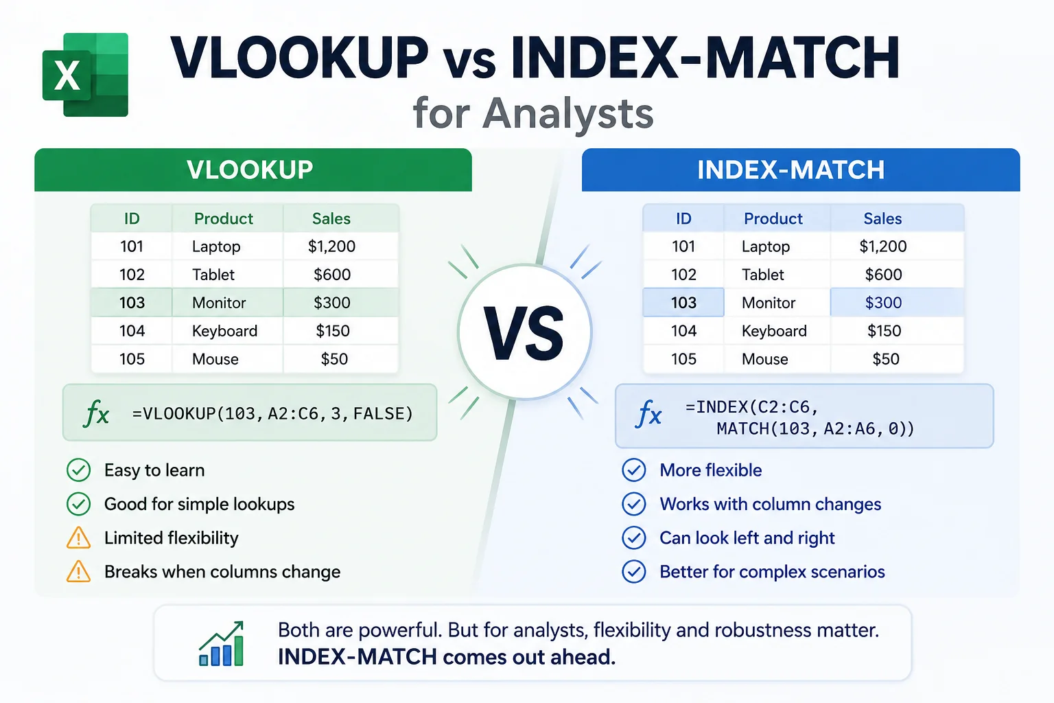
VLOOKUP (Vertical Lookup) works like this: you give it a value to search for, a range to search in, and a column number to pull from. It always searches the leftmost column of your range and returns a value from a column to the right.
=VLOOKUP(lookup_value, table_array, col_index_num, [range_lookup])
INDEX-MATCH is actually two formulas working together. MATCH finds the position of your lookup value in a column or row. INDEX then uses that position to return a value from any range you point it to.
=INDEX(return_range, MATCH(lookup_value, lookup_range, 0))
Yes, INDEX-MATCH looks more complicated. It is — at first. But once it clicks, it's hard to go back to VLOOKUP.
The Case for VLOOKUP: When Simple Wins
Let's not pretend VLOOKUP is bad. It's been the most-used lookup function in Excel for decades, and that's not an accident.
Here's where VLOOKUP genuinely shines.
When your data is clean and simple. If you have a product list with an ID in column A and a price in column B, VLOOKUP is all you need. One formula, easy to read, easy to explain to a coworker.
When you're teaching someone else. VLOOKUP's syntax maps almost directly to plain English: "Look up this value, search in this table, give me column 3." Even a non-Excel person can follow it. INDEX-MATCH? Not so much — at least not on the first read.
When your table won't change. The big gotcha with VLOOKUP is the hardcoded column number. =VLOOKUP(A2, B:D, 2, 0) will always pull from the second column. If someone inserts a column in your table, that number is now wrong and your formula breaks silently. But if your spreadsheet is locked down and no one's going to add columns, this isn't a real problem.
When speed of entry matters. You can type a VLOOKUP formula in about 10 seconds once you know it. INDEX-MATCH takes a bit longer, especially when you're building it from scratch.
The Case for INDEX-MATCH: When Power Matters
Here's where things get interesting.
INDEX-MATCH doesn't just do what VLOOKUP does — it does things VLOOKUP can't do. For anyone doing real data analysis, this matters a lot.
It Can Look Left
This is the big one. VLOOKUP can only look to the right. If your lookup value is in column C and the result you need is in column A, VLOOKUP can't help you without restructuring your data.
INDEX-MATCH doesn't care. You can look in any direction. The lookup column and the return column are completely independent of each other.
Example: You have employee data with Name in column D and Employee ID in column A. You want to find the ID for a specific name. VLOOKUP fails here. INDEX-MATCH handles it in one formula:
=INDEX(A:A, MATCH("Sarah", D:D, 0))
Done.
It Doesn't Break When You Insert Columns
Because MATCH returns a position rather than you hardcoding a column number, adding or deleting columns in your table doesn't break anything. The formula adapts automatically. For any spreadsheet that's actively being edited — which is basically all of them — this is a huge reliability win.
It's Faster on Large Datasets
VLOOKUP searches the entire table range every time. INDEX-MATCH is generally more efficient on large data, especially when MATCH is used with a sorted list and approximate matching. On a few hundred rows, you won't notice. On 100,000+ rows with lots of formulas recalculating, the difference becomes real.
It Handles Multiple Criteria (With a Trick)
Standard VLOOKUP can only match on one column. INDEX-MATCH can be combined with arrays to match on multiple columns simultaneously. For example, finding a sales figure where both the region AND the product name match:
=INDEX(C:C, MATCH(1, (A:A="North") * (B:B="Widget"), 0))
(Enter this as an array formula with Ctrl+Shift+Enter in older Excel versions, or just Enter in Microsoft 365.)
VLOOKUP can't do this natively. Full stop.
Head-to-Head: The Real Comparison
Simple right-to-left lookups: Both handle this fine. VLOOKUP is slightly easier to write here, but INDEX-MATCH works just as well.
Looking left (result left of your lookup column): VLOOKUP fails completely — it can only look to the right. INDEX-MATCH handles it with no workarounds needed.
Surviving column insertions: VLOOKUP breaks silently if someone adds a column to your table, because it relies on a hardcoded column number. INDEX-MATCH points directly at the column by reference, so it stays stable no matter what changes around it.
Matching on multiple criteria: VLOOKUP can't do this natively. INDEX-MATCH can be combined into an array formula to match on two or more columns at once — useful when one column isn't enough to find a unique result.
Beginner-friendly syntax: VLOOKUP wins here. Its logic reads almost like plain English. INDEX-MATCH has a steeper learning curve upfront, though most people get comfortable with it after a few uses.
Performance on large datasets: VLOOKUP scans the entire table range on every lookup. INDEX-MATCH is generally faster on big files, especially when you're running hundreds of formulas at once. On small datasets you won't notice the difference.
Two-way lookup (matching on both a row and a column): VLOOKUP can't do this. INDEX-MATCH can — you use one MATCH to find the row and another to find the column, then INDEX pulls the value at that intersection.
Error handling: Both return a #N/A error when the lookup value isn't found. Wrap either formula in IFERROR to show something friendlier instead.
Read more about Excel Pivot Tables Tutorial: Hands-On Guide for Data Analysis.
The Scenario That Converts Most VLOOKUP Users
I want to walk you through a specific scenario, because this is the one that gets people.
Imagine you're an SMB owner tracking invoices. You have a spreadsheet with:
- Column A: Invoice Number
- Column B: Client Name
- Column C: Amount
- Column D: Status (Paid / Unpaid)
You're using =VLOOKUP(G2, A:D, 4, 0) to pull the status for a given invoice number. It works perfectly.
Then your accountant adds a "Due Date" column between C and D, making Status column 5 now instead of column 4.
Every single VLOOKUP formula in your spreadsheet now returns the wrong value — and shows no error. It just quietly pulls the wrong column. You might not catch it until you've already made a business decision on bad data.
The INDEX-MATCH version?
=INDEX(D:D, MATCH(G2, A:A, 0))
You're pointing directly at column D by reference, not by position. Insert columns all day. It still works.
That scenario — silent wrong data — is the one that convinces most people to switch.
What About XLOOKUP?
Fair question. If you're using Microsoft 365 (the subscription version of Excel), you have access to XLOOKUP, which is a newer function designed to replace VLOOKUP.
XLOOKUP fixes most of VLOOKUP's problems. It can look left, doesn't use column numbers, has better error handling built in, and its syntax is clean. In some ways it's even simpler than INDEX-MATCH for basic tasks.
=XLOOKUP(lookup_value, lookup_array, return_array, [if_not_found])
So should you just learn XLOOKUP instead?
Here's the honest answer: if you're on Microsoft 365 and only working with your own files, yes — XLOOKUP is fantastic. But there's a catch. XLOOKUP doesn't exist in Excel 2019, Excel 2016, or Google Sheets. If you share files with clients or colleagues who aren't on 365, your XLOOKUP formulas will show as errors on their end.
INDEX-MATCH works everywhere. It's been in Excel since the 1990s. It works in Google Sheets. It works in older Excel versions. For anyone working across different environments or sharing files widely, INDEX-MATCH is still the most universally compatible powerful lookup option.
VLOOKUP vs INDEX-MATCH remains the relevant comparison for a huge portion of real-world Excel users.
A Quick INDEX-MATCH Tutorial for Beginners
If you've never written INDEX-MATCH before, here's how to build it step by step without getting overwhelmed.
Step 1: Write the MATCH part first.
MATCH answers one question: "What row is my value in?"
=MATCH("Apple", A:A, 0)
This says: find "Apple" in column A, and give me its row number. The 0 at the end means exact match (you almost always want 0).
Run this formula on its own first. It should return a number, like 7. That means "Apple" is in row 7.
Step 2: Add INDEX around it.
INDEX answers: "Given a row number, what value is in that row in a different column?"
=INDEX(B:B, 7)
This returns whatever is in row 7 of column B.
Step 3: Combine them.
Instead of hardcoding 7, let MATCH find the row number automatically:
=INDEX(B:B, MATCH("Apple", A:A, 0))
And that's it. That's the whole thing. INDEX uses whatever row number MATCH finds.
Once you've written it a few times, it becomes second nature. The key insight is that MATCH gives you a position, and INDEX uses that position to grab a value.
Common Mistakes (And How to Fix Them)
Mistake 1: Getting #N/A errors
This usually means the lookup value wasn't found. Check for extra spaces (trim your data with =TRIM()), mismatched data types (numbers stored as text is a classic), or typos in the lookup value.
Wrap with IFERROR to handle gracefully:
=IFERROR(INDEX(B:B, MATCH(G2, A:A, 0)), "Not Found")
Mistake 2: Forgetting the 0 in MATCH
=MATCH(value, range, 0) means exact match. Without the 0, Excel uses approximate match by default, which requires sorted data and often returns wrong results. Always include the 0 unless you specifically need approximate matching.
Mistake 3: Using entire columns when the dataset is huge
INDEX(A:A, MATCH(..., B:B, 0)) works, but referencing entire columns in very large files can slow things down. Locking to a specific range like INDEX(A2:A10000, MATCH(..., B2:B10000, 0)) is better practice for performance.
Mistake 4: Column/row mismatch
Make sure your INDEX range and your MATCH range have the same number of rows (for vertical lookups). If MATCH searches 500 rows but INDEX only covers 100, you'll get wrong results or errors.
Who Should Use What
Stick with VLOOKUP if:
- You're new to Excel lookup functions and want to learn the basics first
- Your data is simple, stable, and you only ever need to look right
- You're building a quick one-off spreadsheet that no one else will maintain
- You're explaining something to a non-Excel person and need it to be readable
Switch to INDEX-MATCH if:
- You're doing serious data analysis or building spreadsheets others will use long-term
- Your data structure might change (new columns, new rows)
- You need to look left, match on multiple criteria, or do two-way lookups
- Performance matters because you have large datasets
- You're working across different Excel versions or Google Sheets
Learn XLOOKUP too if:
- You're on Microsoft 365 and mostly working within your own files
- You want the simplest possible syntax for modern Excel
The honest recommendation: learn VLOOKUP to understand the concept, then invest a couple of hours getting comfortable with INDEX-MATCH. That investment pays off every single week.
The Bottom Line
VLOOKUP isn't obsolete. It's quick, it's readable, and it gets the job done for basic lookups. But it has real limitations that bite you exactly when it matters on large, changing, real-world spreadsheets.
INDEX-MATCH takes about an hour to learn properly. After that, it handles every situation VLOOKUP can, plus a dozen situations VLOOKUP can't. For anyone doing regular data work, it's the better long-term investment.
Related: Fine-Tune a Small LLM on Your Own Data in 2026: A Step-by-Step Guide
Here's the thing: you don't have to choose forever. VLOOKUP for quick, simple lookups in stable spreadsheets. INDEX-MATCH for anything serious. That's a perfectly reasonable approach.